TT14 -2023: Premier League Match Data 2021-2022

tidytuesday
Autor/a

Benjamín Adasme Jara

Fecha de publicación

4 de abril de 2023

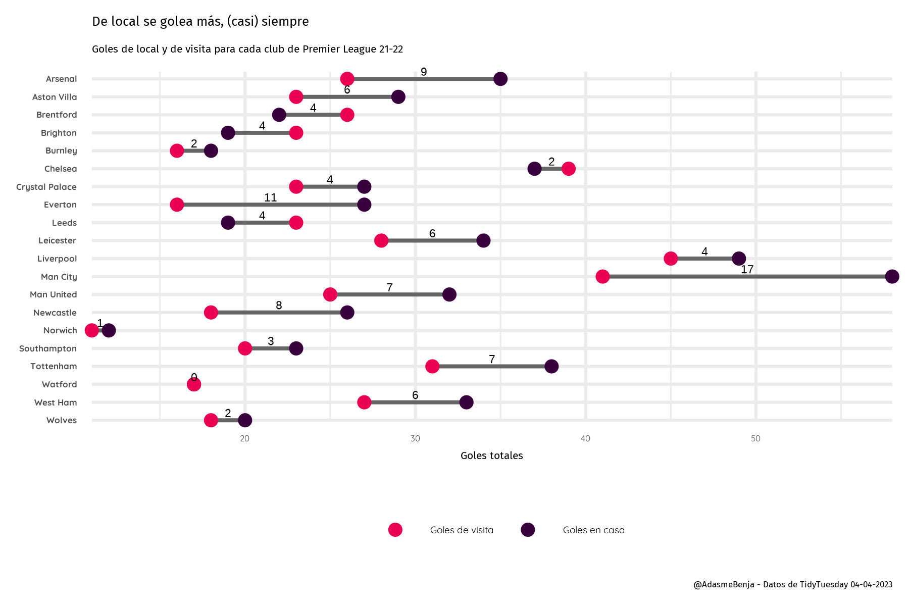
En esta edición de Tidy Tuesday del 04 de abril de 2023 trabajamos con los datos de la Premier League temporada 2021-2022, donde nos entrega la data de cada partido y sus resultados. Con esto, quisimos consultar la cantidad de goles de local y de visita de cada equipo, para saber si la capacidad goleadora se ve afectada por el estadio.

Resultado

Código

Cargamos los paquetes y los datos

pacman::p_load(tidyverse,
               tidytuesdayR,
               lubridate, 
               showtext)

data_14 <- tt_load("2023-04-04")
---- Compiling #TidyTuesday Information for 2023-04-04 ----
--- There is 1 file available ---


── Downloading files ───────────────────────────────────────────────────────────

  1 of 1: "soccer21-22.csv"
epl_21_22 <- data_14$`soccer21-22`

Luego, cargamos las fuentes elegidas para este gráfico

font_add_google("Fira Sans", "fira")
font_add_google("Quicksand", "quick")
showtext_auto()

Calculamos la cantidad de goles, tiros y tiros apuerta de los equipos locales y los equipos visitantes.

home_goals <- epl_21_22 %>% 
  group_by(HomeTeam) %>% 
  summarise(home_goals = sum(FTHG),
            home_shots = sum(HS),
            home_shot_target = sum(HST))

away_goals <- epl_21_22 %>% 
  group_by(AwayTeam) %>% 
  summarise(away_goals = sum(FTAG),
            away_shots = sum(AS),
            away_shot_target = sum(AST))

head(home_goals)
# A tibble: 6 × 4
  HomeTeam    home_goals home_shots home_shot_target
  <chr>            <dbl>      <dbl>            <dbl>
1 Arsenal             35        347              116
2 Aston Villa         29        235               86
3 Brentford           22        233               77
4 Brighton            19        280               67
5 Burnley             18        229               73
6 Chelsea             37        326              115

Unimos los resultados de ambas tablas en una sola consolidada

tot_goal_shot <- home_goals %>% 
  left_join(away_goals, by = c("HomeTeam" = "AwayTeam")) %>% 
  rename("Team" = HomeTeam)

head(tot_goal_shot)
# A tibble: 6 × 7
  Team        home_goals home_shots home_shot_target away_goals away_shots
  <chr>            <dbl>      <dbl>            <dbl>      <dbl>      <dbl>
1 Arsenal             35        347              116         26        241
2 Aston Villa         29        235               86         23        219
3 Brentford           22        233               77         26        209
4 Brighton            19        280               67         23        210
5 Burnley             18        229               73         16        178
6 Chelsea             37        326              115         39        266
# ℹ 1 more variable: away_shot_target <dbl>

Creamos el dataset segmentos que permite dibujar las líneas entre puntos.

segmentos <- tot_goal_shot %>% 
  select(c(Team, home_goals, away_goals)) %>% 
  mutate(goal_dif = home_goals - away_goals,
         Team = fct_reorder(Team, desc(Team)))
# levels(segmentos$Team)

head(segmentos)
# A tibble: 6 × 4
  Team        home_goals away_goals goal_dif
  <fct>            <dbl>      <dbl>    <dbl>
1 Arsenal             35         26        9
2 Aston Villa         29         23        6
3 Brentford           22         26       -4
4 Brighton            19         23       -4
5 Burnley             18         16        2
6 Chelsea             37         39       -2

Luego selecciinamos solo los goles, reordenamos los equipos para que aparezcan alfabéticamente, y modificamos la forma de la tabla, para que quede en un formato “long”.

tot_long <- tot_goal_shot %>% 
  select(c(Team, home_goals, away_goals)) %>% 
  mutate(Team = fct_reorder(Team, desc(Team))) %>% 
  pivot_longer(cols = 2:3, names_to = "H_A", values_to = "goals")

head(tot_long)
# A tibble: 6 × 3
  Team        H_A        goals
  <fct>       <chr>      <dbl>
1 Arsenal     home_goals    35
2 Arsenal     away_goals    26
3 Aston Villa home_goals    29
4 Aston Villa away_goals    23
5 Brentford   home_goals    22
6 Brentford   away_goals    26

Pasamos el dataset en formato “long” a ggplot2 y configuramos todos los detalles.

tot_long %>% 
  ggplot(aes(y = Team, group = Team)) +
  geom_segment(data = segmentos,
               aes(x = home_goals, xend = away_goals, yend = Team),
               color = "gray40", 
               linewidth = 0.9) +
  geom_point(aes(x = goals, color = H_A), size = 2.5) +
  geom_text(data = segmentos,
            aes(y = Team, x = (away_goals + goal_dif*0.5), label = abs(goal_dif)),
            position = position_nudge(y = 0.4),
            size = 6) +
  scale_color_manual(values = c("#e90052", "#38003c"), # Colores oficiales PL 
                     labels = c("Goles de visita", "Goles en casa"),
                     name = NULL) +
  labs(x = "Goles totales", y = NULL, caption = "@AdasmeBenja - Datos de TidyTuesday 04-04-2023",
       title = "De local se golea más, (casi) siempre", 
       subtitle = "Goles de local y de visita para cada club de Premier League 21-22") +
  coord_cartesian(expand = F,
                  clip = "off") +
  theme_minimal(base_family = "quick", base_size = 16) +
  theme(
    #plot.background = element_rect(fill = "#07F2F2"), 
        title = element_text(family = "fira"),
        axis.text.y = element_text(face = "bold"),
        legend.position = "bottom",
        legend.direction = "horizontal",
        legend.text = element_text(size = 14)#,
        # legend.key.size = unit(0.5, "cm")
        )

Guardamos el gráfico como imágen para exportar y compartir.

ggsave("2023-w14-premierleague2.jpg", dpi = 300, width = 6, height = 4)